Electric Potential -

Electric Potential

We know that electric field intensity is the force per unit test charge, similarly electric potential is defined as the potential energy per unit test charge.

i.e. potential at a point is defined as

$\fn_cm \mathbf{\left [ V=\frac{U}{q} \right ]}\;\;\;or\;\;\;\mathbf{\left [ V=\frac{W_{ext}}{q} \right ]}$

Hence ” Electric potential at a point in an electric field is the amount of work done in moving a unit +ve charge slowly from infinity to that point against electric force.”

Electric Potential is a scalar quantity and its S.I unit is J/C or Volt.

NOTE:-

(1) Electric field strength can be described in terms of either vector $\fn_cm \vec{E}$ or scalar V

(2) The potential energy of charge $\fn_cm q$ at a point where the potential is $\fn_cm V$ is given by $\fn_cm \left [ U=qV \right ]$

(3) Electric potential difference: The potential difference between two points is an electric field is the amount of work done in bringing a unit +ve charge from one point to another.

i.e. $\fn_cm \left [ V_B-V_A=\frac{W_{A\rightarrow B}}{q} \right ]\;\;\;\;\;\Rightarrow \;\;\;\;\;\left [ W_{A\rightarrow B}=q(V_B-V_A) \right ]$

(4) A common unit of P.E. in atomic physics is eV. $\fn_cm \left [ 1eV=1.6\times 10^{-19}J \right ]$ . It is the amount of work done when an electron is moved through a p.d. of 1 volt.

(5) if $\fn_cm W_{A\rightarrow B}>0,$ then $\fn_cm V_B>V_A$

i.e. B is at a higher potential and A is at a lower potential (L→H)

if $\fn_cm W_{A\rightarrow B}=0,$ then $\fn_cm V_B=V_A$

if $\fn_cm W_{A\rightarrow B}<0,$ then $\fn_cm V_B<V_A$

i.e. A is at a higher potential and B is at a lower potential (H→L)

(6) +ve charge always flows from higher potential to lower potential.

Electric potential at a point due to a single-point charge

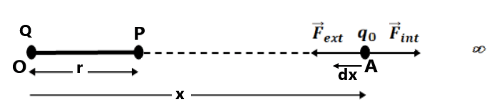
Consider a point charge Q placed at point O. We have to calculate electric potential at point P which is distance r from O. Consider a point A intermediate between ∞ and P.

The electric field on $\fn_cm q_0$ at A due to Q is

$\fn_cm F_{int}=\frac{kQq_0}{x^2}$

∴ external force is the same as $\fn_cm F_{int}$ but in the opposite direction.

i.e. $\fn_cm F_{ext}=\frac{kQq_0}{x^2}$

∴ work done by this force due to small displacement dx is

$\fn_cm dW=\vec{F}_{ext}.d\vec{x}$

$\fn_cm =-F_{ext}dx \cos0^0$ (here -ve sign is taken because dx is measured along the -ve direction of x)

$\fn_cm dW=-\frac{kQq_0}{x^2}dx$

∴ Total work done in moving the charge $\fn_cm q_0$ from ∞ to the point P will be

$\fn_cm W=-kQq_0\int_{\infty}^{r}\frac{1}{x^2}dx$

$\fn_cm W=-kQq_0\left [- \frac{1}{x^2} \right ]_{\infty}^r$

$\fn_cm W=-kQq_0\left [- \frac{1}{r}+\frac{1}{\infty} \right ]$

$\fn_cm \left [ W=\frac{kQq_0}{r} \right ]$

∴ The electric potential at point P is defined as

$\fn_cm V=\frac{W}{q_0}$

$\fn_cm \mathbf{\left [ V=\frac{kQ}{r} \right ]}$

Note:-

1. If a medium is introduced, the potential at a point is defined as

$\fn_cm \left [ V=\frac{1}{4\pi\epsilon_0}\frac{Q}{kr} \right ]$

where $\fn_cm k\rightarrow$ dielectric constant

2. at $\fn_cm r\rightarrow \infty, V\rightarrow 0$

i.e. at infinite, electric potential is zero

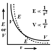
3. For a point charge $\fn_cm V \propto \frac{1}{r^2}\;\;\;and\;\;\;E \propto \frac{1}{r^2}$ therefore, the electric field intensity $\fn_cm E$ decreases more rapidly than potential $\fn_cm V$ with increasing distance $\fn_cm r$ .

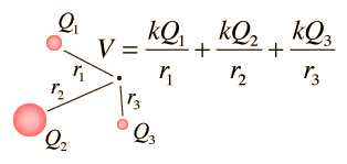
4. Potential at a point due to a group of point charges

5. The potential near the +ve charge is more than the potential near the -ve charge.

6. Potential due to +ve charge decreases with increasing distance and potential due to -ve charge increases with increasing distance and vice versa.

7. Potential at a point due to continuous charge distribution. ( Use Integration technique)

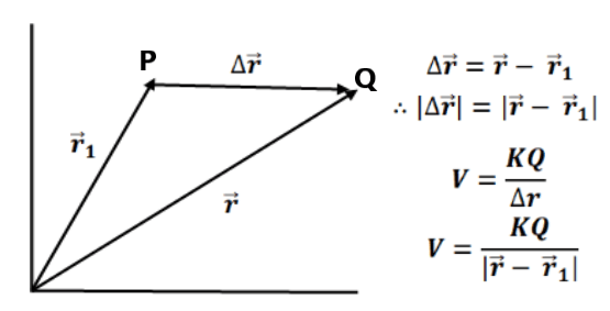
8. Potential in vector form.

Potential of charges in an external electric field

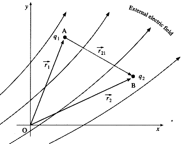
Let us consider two point charges $\fn_cm q_1$ and $\fn_cm q_2$ placed at points A and B in an external electric field. They are at a distance of $\fn_cm r_1$ and $\fn_cm r_2$ from the origin. Let the potential at A is $\fn_cm V(r_1)$ and potential at B is $\fn_cm V(r_2)$ respectively.

i.e. work done in bringing a charge $\fn_cm q_1$ from $\fn_cm \infty$ to point A inside the external electric field is

$\fn_cm W_1=q_1V(r_1)$

This is the P.E of charge $\fn_cm q_1$ in the external electric field

i.e. $\fn_cm U_1=q_1V(r_1)$

Similarly, the P.E of charge $\fn_cm q_2$ in an external electric field is

$\fn_cm U_2=q_1V(r_2)$

Total P.E of system = Workdone is assembling the two charges

$\fn_cm \mathbf{\left [ U=q_1V(r_1)+q_2V(r_2)+\frac{kq_1q_2}{r_{21}} \right ]}$

Electric potential due to an electric dipole

Case 1: On the axial line

at P $\fn_cm V_P=V_A+V_B$

$\fn_cm =\frac{kq}{(r-d)}-\frac{kq}{(r+d)}$

$\fn_cm =kq\left [ \frac{r+d-r+d}{r^2-d^2} \right ]$

$\fn_cm =\frac{kq2d}{r^2-d^2$

$\fn_cm \left [ V_P=\frac{kP}{r^2-d^2} \right ]$

$\fn_cm if\;\;r>>d,\;\;then\;\;(r^2-d^2\)\approx r^2$

$\fn_cm \left [ V_p=\frac{KP}{r^2} \right ]$

Case 2: On the equatorial line

at P $\fn_cm V_P=V_A+V_B$

$\fn_cm V_P=\frac{kq}{\sqrt{r^2+d^2}}-\frac{kq}{\sqrt{r^2+d^2}}$

$\fn_cm \left [ V_P=0 \right ]$

Case 3: At any point

Consider a small dipole AB consisting of two charges -q and +q- separated by a small distance 2d. We have to calculate electric potential at any point P which is distance r from center of dipole O.

Let $\fn_cm \angle POB=\theta$

from the figure, suppose $\fn_cm AP=r_1\;\;and \;\;BP=r_2$

Draw $\fn_cm BD \perp OP\;\;\;and\;\;\;AC \perp OP$

$\fn_cm here\;\;\;r_1\approx CP=OP+OC=r+d\cos\theta$

$\fn_cm also\;\;\;r_2\approx DP=OP-OD=r-d\cos\theta$

Now potential at P due to dipole is

$\fn_cm V_P=\frac{kq}{r_2}-\frac{kq}{r_1}=kq\left [ \frac{1}{r_2}-\frac{1}{r_1} \right ]$

$\fn_cm =kq\left [ \frac{1}{r-d\cos\theta}-\frac{1}{r+d\cos\theta} \right ]$

$\fn_cm =kq\left [ \frac{r+d\cos\theta-r+d\cos\theta}{r^2-d^2cos^2\theta} \right ]$

$\fn_cm =\frac{kq2d\cos\theta}{r^2-d^2\cos^2\theta}$

$\fn_cm \left [ V_P=\frac{kP\cos\theta}{r^2-d^2\cos^2\theta} \right ]$

$\fn_cm \because r>>>d\;\;\;\therefore \;\;\;r^2-d^2\cos^2\theta \approx r^2$

$\fn_cm \left [ V_P=\frac{kP\cos\theta}{r^2} \right ]$

Special Case

(a) When point P lies on the axial line i.e. θ=0° or 180°

$\fn_cm i.e. \;\;\;V_P=\frac{kP\cos0^0}{r^2}\;\;\;or\;\;\; \frac{kP\cos180^0}{r^2}$

$\fn_cm \left [ V_P=\frac{kP}{r^2}\;\;\;or\;\;\; \frac{-kP}{r^2} \right ]$

(b) When point P lies on the equatorial line i.e. θ=90°

$\fn_cm i.e.\;\;\;\theta=90^0$

$\fn_cm V_P=\frac{kP\cos90^0}{r^2}\;\;\;\Rightarrow \;\;\;\left [V_P=0 \right ]$

NOTE:-

$\fn_cm \mathbf{1.}$ The electric potential due to point charge is $\fn_cm \left ( V\propto \frac{1}{r} \right )$ while for dipole $\fn_cm \left ( V\propto \frac{1}{r^2} \right )$ . Thus the electric potential due to dipole decreases quickly with an increase in distance compared to the potential due to a point charge.

$\fn_cm \mathbf{2.}$ The potential due to a dipole is axially symmetric. If we rotate the observation point P about the dipole axis (keeping r and θ fixed), the potential doesn’t change. However potential due to a point charge is spherically symmetric.

Relation between electric field and electric potential

Suppose, the electric field at a point due to a charge distribution is $\fn_cm \vec{E}$ and the electric potential at the same point is V.

Let a point charge $\fn_cm q$ is placed at that point. Force on charge $\fn_cm q$ is $\fn_cm \vec{F}=q\vec{E}$

Suppose, due to this force, the charge $\fn_cm q$ is displaced slightly $\fn_cm d\vec{r}$ . The work done by electric force (internal force) during this displacement is

$\fn_cm dW=\vec{F}.d\vec{r}=q\vec{E}.d\vec{r}$

By definition, a change in potential energy is given by

$\fn_cm dU=-dW_{int}$

$\fn_cm i.e. \;\;\;dU=-q\vec{E}.d\vec{r}$

we know that $\fn_cm dV=\frac{dU}{dr}$

$\fn_cm \therefore \;\;\; dV=-\frac{q\vec{E}.d\vec{r}}{q}$

$\fn_cm \left [ dV=-\vec{E}.d\vec{r} \right ]$

This is the relation between V and E.

Here we can also write

$\fn_cm \left [ dV=-Edr\cos\theta \right ]$ where θ is the angle between $\fn_cm \vec{E}$ and $\fn_cm d\vec{r}$

Now, $\fn_cm -\frac{dV}{dr}=E\cos\theta$ Gives the component of the electric field in the direction of $\fn_cm d\vec{r}$ .

$\fn_cm \frac{dV}{dr}\rightarrow$ Potential gradiant, it is the rate of change of potential with r. -ve sign indicate, V is decreasing in the direction of E.

if $\fn_cm \theta=0^0$ , $\fn_cm \;\;\; then\left [ -\frac{dV}{dr}=E \right ]\;\;\; is\;\;\; maximun$

i.e., the electric field is along the direction in which the potential decreases at the maximum rate.

From the above relation S.I. unit of an electric field is V/m.

If work done is on the cartesian system, then

$\fn_cm \vec{E}=E_x\hat{i}+E_y\hat{j}+E_z\hat{k}\;\;\;and\;\;\; d\vec{r}=dx\hat{i}+dy\hat{j}+dz\hat{k}$

and we can write

$\fn_cm dV=-\vec{E}.d\vec{r}$

$\fn_cm dV=(E_x\hat{i}+E_y\hat{j}+E_z\hat{k}) .(dx\hat{i}+dy\hat{j}+dz\hat{k})$

$\fn_cm \left [ dV=-E_x dx-E_ydy-E_zdz \right ]$

if y and z are constant, then $\fn_cm \partial V=-E_x\partial x$

if z and x are constant, the $\fn_cm \partial V=-E_y\partial y$

if x and y are constant, then $\fn_cm \partial V=-E_z\partial z$

otherwise

$\fn_cm V=-\left [ \int_{x_1}^{x_2} E_xdx+\int_{y_1}^{y_2} E_ydy+\int_{z_1}^{z_2} E_zdz\right ]$

* In uniform electric field

Case 1:-

$\fn_cm \int_{V_A}^{V_B}dV=-\int_0^d \vec{E}.d\vec{r}$

$\fn_cm here\;\; \theta=0^0$

$\fn_cm V_B -V_A= -\int_0^d Edr\cos0^0$

$\fn_cm V_B-V_A=-Ed$

$\fn_cm \therefore V_A-V_B=Ed$

i.e. Potential drop is $\fn_cm \left [ V=Ed \right ]$

Case 2:-

$\fn_cm \int_{V_A}^{V_B}dV=-\int_0^d \vec{E}.d\vec{r}$

$\fn_cm here\;\; \theta=90^0$

$\fn_cm V_B -V_A= -\int_0^d Edr\cos90^0$

$\fn_cm V_B-V_A=0$

$\fn_cm \left [ V_A=V_B \right ]$

Finding electric field, if potential is given

We know that

$\fn_cm \left [ dV=-E_x dx-E_ydy-E_zdz \right ]$

if x co-ordinate is changed from x to x+dx keeping y and z co-ordinate unchanged i.e. dy=dz=0

$\fn_cm \therefore \;\; \partial V=-E_x\partial x\;\;\; \Rightarrow \;\;\; \left [ E_x=-\frac{\partial V}{\partial x} \right ]$

Similarly,

$\fn_cm \left [ E_y=-\frac{\partial V}{\partial y} \right ]$ and $\fn_cm \left [ E_z=-\frac{\partial V}{\partial z} \right ]$

and we can write

$\fn_cm \left [ \vec{E}=E_x\hat{i}+E_y\hat{j}+E_z\hat{k} \right ]$

Finding potential if electric field is given

Here we can use only

$\fn_cm \left [ dV=-\vec{E}.d\vec{r} \right ]\;\;\; \Rightarrow \;\;\; \left [ \int dV=-\int \vec{E}.d\vec{r} \right ]$

Equipotential surface

Any surface which has the same potential at every point is called an equipotential surface.

Properties of equipotential surface:-

1. The potential difference between any two points of any equipotential surface is zero

2. No work is done in moving a test charge over an equipotential surface.

3. Electric field is always perpendicular to the equipotential surface.

4. Two equipotential surface can never intersect because at the point of intersection there are two values of potential which is impossible.

5. The spacing between equipotential surface enables us to identify region of strong and weak fields.

Electric field due to continuous charge distribution

Self Energy

Earting of a conductor

Behaviour of conductor in electric field