The electric field due to a charge is the space around the charge in which any other charge experiences a force of attraction or repulsion.
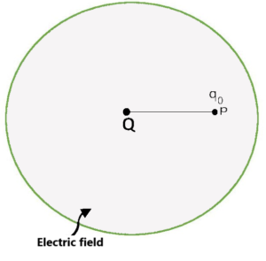
Theoretically, an electric field due to a charge extends up to infinity. However, the effect of the electric field dies (vanish) quickly as the distance from the charge is increased.
The strength of an electric field is described by a quantity called electric field intensity or electric field strength. It is defined as the force experienced by unit +ve charge placed at that point or force experienced per unit test charge (). It is denoted by E.
i.e.
It is a scalar quantity and its direction is same as force. Its S.I unit is N/C or V/m
Electric field intensity at a point due to a point charge
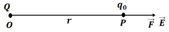
From figure,
force on due to
is given by
From the definition, an electric field at a point P is given by
Its magnitude will be
NOTE
(1) The magnitude of electric field strength depends upon the magnitude of charge which produces the electric field and not on the value of the test charge
.
(2) Electric field at a point due to group of a point charges ( Superposition principle)
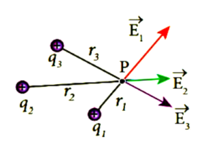
The net electric field strength at point P is
(3) If any charge () is placed at a point where electric field strength is
, then force experienced by
is given by
(4) A charged particle is not affected due to its own field.
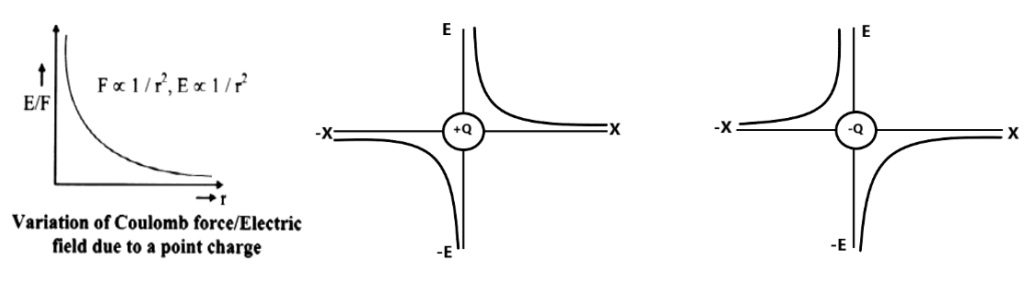
(5) Variation of E due to point charge.
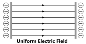
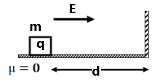
(6) UNIFORM ELECTRIC FIELD:- A space where the electric field is uniform, means the magnitude and direction of electric field strength are the same at every point in space.
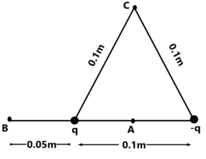
EXERCISE 1(1) Determine the electric field vector at a distance of 0.50 m from a charge of -2μC. ( (2) Two point charges (a) The midpoint between the charges. ( (b) A point on the line joining (3) Two point charges of +16μC and -9μC are placed 8 cm apart in the air. Determine the position of the point at which the resultant field is zero. (24 cm to the right of -9μC ) (4) Calculate the electric field at points A, B, and C as shown in fig. where
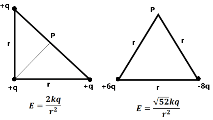
(5) Find the electric field at point P as shown in the figure.
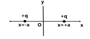
(6) Two identical positive point charges
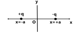
(a) Plot the variation of E along the X-axis. (b) Plot the variation of E along the Y- axis. (7) Plot the variation of E along X-axis and Y-axis for the charge distribution as shown in the figure.
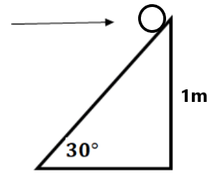
(8) Two-point charges (9) An inclined plane making an angle of 30° with the horizontal is placed in a uniform horizontal electric field of 100 N/C. A particle of mass 1 kg and charge 0.01C is allowed to slide down from rest from a height of 1m. If the co-efficient of friction is 0.2, find the time taken by the particle to reach the bottom. take g=9.8 m/s².
(10) the position vector of two point charges (11) A point charge of (12) Two point charges (a) What is the electric field at the midpoint of the line joining the two charges? ( (b) If a -ve test charge of magnitude (13) ABCD is a square of side 5m. Charges of +50μC, -50μC and +50μC are placed at A , C and D respectively. Find the resultant electric field at B. (14) Four charges +q,+q,-q,-q are placed respectively at the four corners A, B, C and D of a square of side ‘a’. Calculate the electric field at the centre of the square. |
Electric Line of Force / Electric Fields Lines
It is useful to have a kind of “map” that gives the direction and strength of the field at various places. Electric field lines, a concept introduced by Michael Faraday (1791-1867) provide us with an easy way to visualize the electric field. It is an imaginary line but the field is real.
“An electric field line is the path along which a small +ve test charge would move slowly when it is free to do so. ”

Properties of Electric Field Lines
(1) Field lines are continuous curves without any breaks.
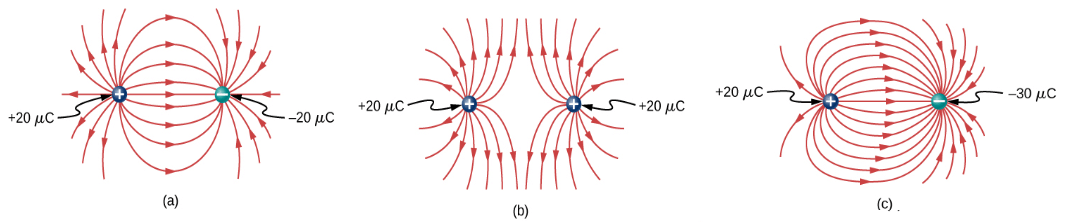
(2) The lines of force start at +ve charges and terminate at -ve charges. If there is a single charge, then the lines of force will start or end at infinity.
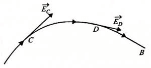
(3) the tangent to a line of force at any point gives the direction of the net electric field at that point.
(4) No two lines of force can cross each other.
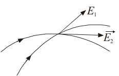
REASON:- If they intersect, then there will be two tangents at that point of intersection and hence two directions of the electric field at the same point, which is not possible.
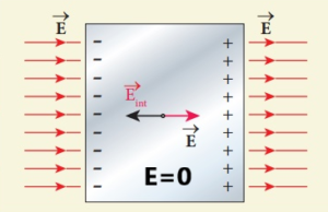
(5) Electric lines of force are always perpendicular to the surface of a conductor.
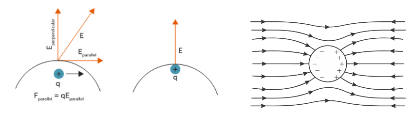
REASON:- If the line of force is not normal to the conductor, the component of the field parallel to the surface would cause the electron to move and would set up a current on the surface. but no current flows in electrostatic.
(6) Electric field lines do not form a closed loop.
REASON:- Because if they do so, then the work done along a closed path will not be zero, which contradicts in conservative nature of the electric field.
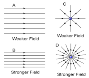
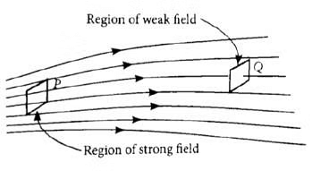
(7) The relative closeness of field lines gives the strength of the electric field.
(8) Electric line of force does not pass through the conductor but passes through an insulator.
(9) Electric field strength at a point is proportional to the number of lines passing through normally per unit area. i.e. it is proportional to the flux density.
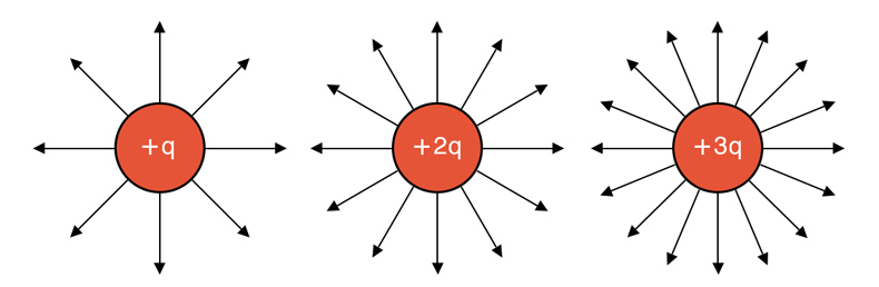
(10) The number of lines coming from or coming to a charge is proportional to the magnitude of charges.
NOTE:
To sketch field lines, pay attention to the following three important points (a) Symmetry (b) Near and far points and (c) The number of lines
EXERCISE 2(1) Calculate the electric field strength required to just support a water droplet of mass (2) A Positively charged oil drop is prevented from falling under gravity by applying a vertical electric field of 100 V/m. If the mass of the drop is (3) A stream of electrons moving with a velocity of (4) A pendulum of mass 80 milligrams carrying a charge of (5) A simple pendulum consists of a small sphere of mass m suspended by a thread of length L. The sphere carries a positive charge q. The pendulum is placed in a uniform electric field of strength E directed vertically downwards. Find the period of oscillation of the pendulum due to the electrostatic force acting on the sphere, neglect the effect of the gravitational force. (6) An uniform electric field
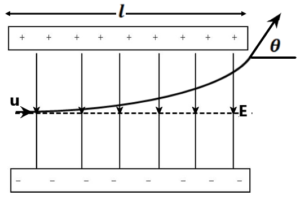
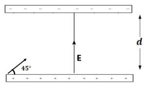
(7) An electron is projected as in Fig with kinetic energy K, at an angle of 45° between two charged plates. Find the magnitude of the minimum electric field so that the electron just fails to strike the upper plate. (E=k/2qd)
(8) A particle of charge q and mass m moves rectilinearly under the action of an electric field (9) A charged cork ball of mass (10) The bob of a simple pendulum has mass m and carries a charge q on it. The length of the pendulum is L. There is a uniform electric field E in the region. Calculate the time period of small oscillation for the pendulum about its equilibrium position in the following case. (a) E is vertically down having magnitude E=mg/q (11)
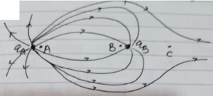
A horizontal electric field towards the right is switched on. Assume elastic collision. Find the time period of the resulting oscillatory motion. Is it a SHM? (12) A particle of mass m and charge q is thrown at a speed u against a uniform electric field E. How much distance will it travel before coming to momentary rest? (13) The field lines for two-point charges as shown in figure.
(a) Is the field uniform? (14) An oil drop of 12 excess electrons is held stationary under a constant electric field of (15) A uniform electric field E exist between two metal plates, one -ve and the other +ve. The plate length is L and the separation of the plates is d. (a) An electron and proton start from the -ve plate and +ve plate respectively and go to opposite plates. which one of them wins this race? |
Stable and Unstable equilibrium
The equilibrium of any body of the system means net force and net torque on it must be zero.
After displacing the charged particle from its equilibrium position, if it returns to its mean position due to restoring force, then it is said to be in stable equilibrium, otherwise it is in unstable equilibrium. (at null point E=0)
The potential energy of stable equilibrium is minimum while that of unstable it is maximum.
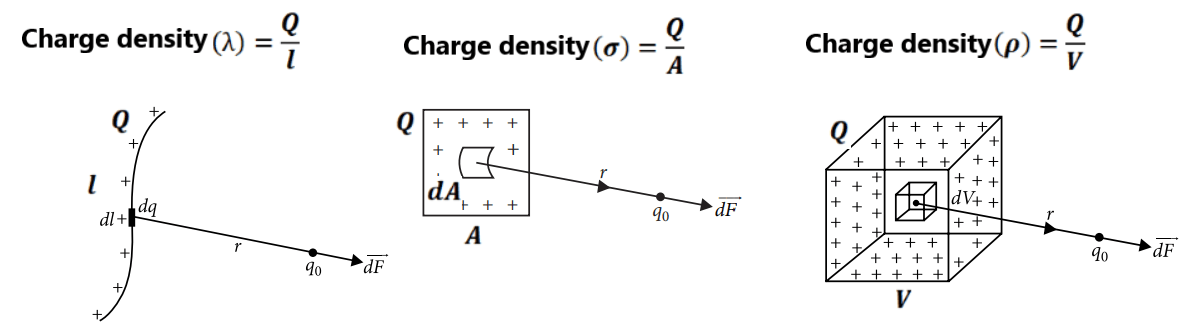
Electric force/ field due to continuous charge distribution:-
Continuous charges can be distributed on the body either along a line, over a surface or a volume depending upon the shape of the body. When we calculate the force/ field by a continuous distribution of charge, this body consists of a very large number of point charges dq.
The total force/ field due to a small point charge dq is calculated at a point. The force due to the entire charge distribution is found by the integration method.
Charge density:- Charge per unit length/ area/ volume depending upon the distribution of charge.
Exercise 3(1) A metal cube of length 0.1 m is charged by 12μC. Calculate its surface charge density. (2) A uniformly charged sphere carries a total charge of (3) Two equal spheres of water having equal and similar charges coalesce to form a large sphere. If no charge is lost, how will the surface charge densities of electrification change? (4) 64 drops of radius 0.02 m and each carrying a charge of 5μC are combined to form a bigger drop. Find how the surface charge density of electrification will change if no charge is lost. (5) Charge is distributed non-uniformly on line such that linear charge density is given as (6) Charge is distributed non-uniformly on a disc such that surface charge density is given as (7) Charge is distributed non-uniformly on a sphere such that volume charge density is given as (8) Find the electric field at point P as shown in the figure.
|
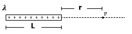
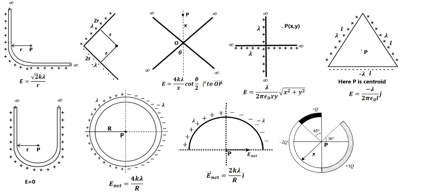
1. Electric field due to line charge
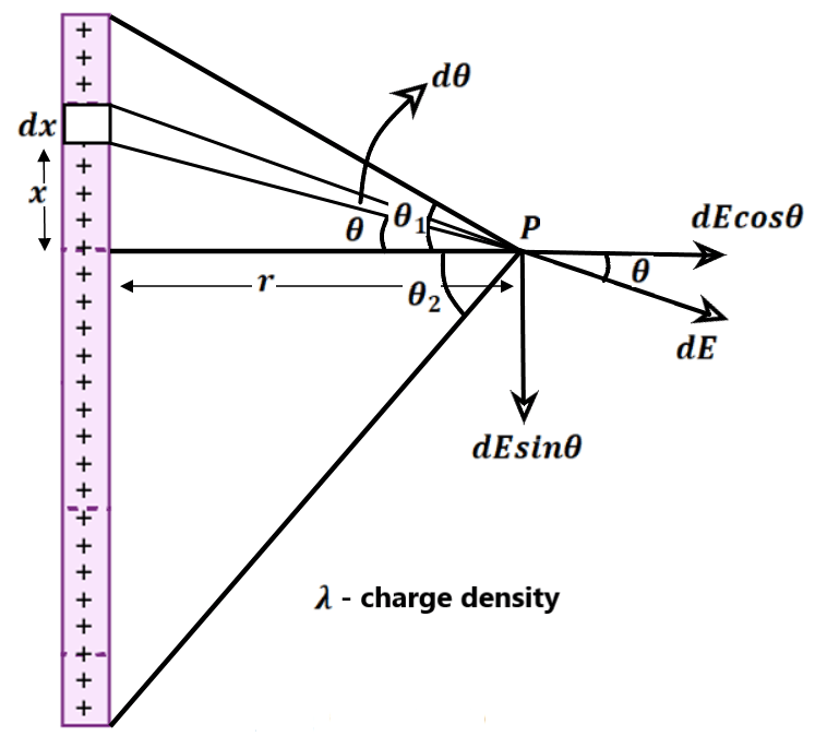
| Let λ is the linear charge density of line. Take small strip of length dx as shown in figure
|
∴ The net electric field at point P is given by
|
Special Case:-
(a) For equatorial position
Here
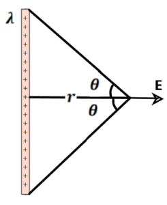
(b) For semi-infinite wire
here
i.e.
and
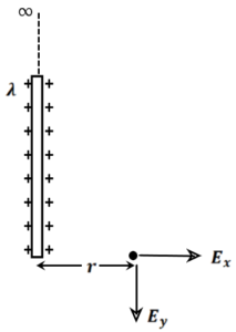
(c) For infinite wire
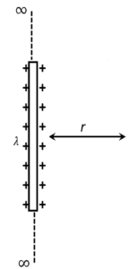
here
(d) Example
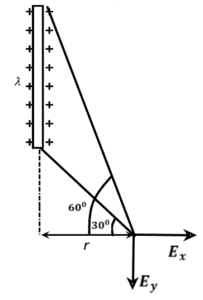
Here take and
(in derivation
was anticlockwise but here is clockwise so we take
-ve)
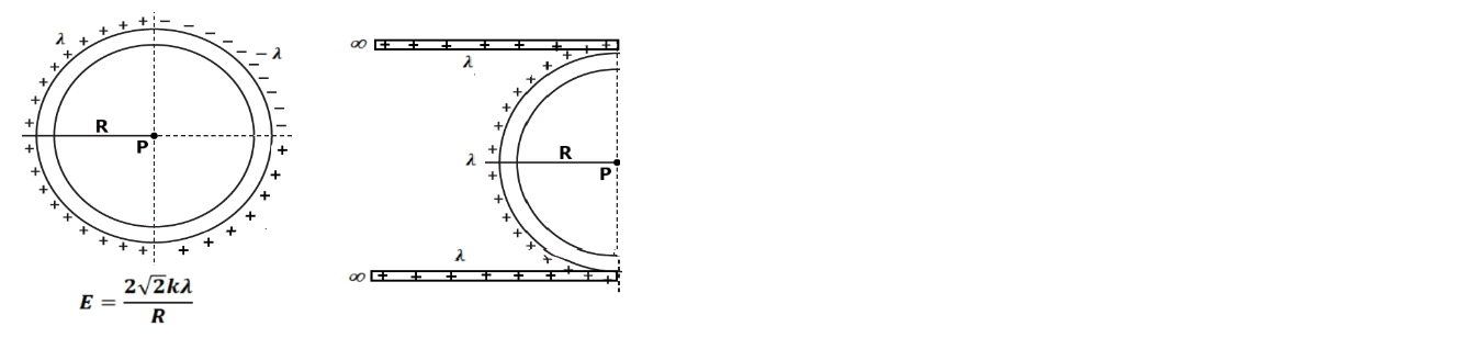
2. Electric field at the centre due to charged circular arc
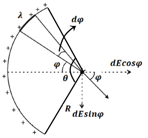
Let linear charge density, then
from figure
The net electric field at a point P ( Centre) is given by
Special Case:
(a) For Quadrant
(b) For semi-circle
(c) For complete circle
3. Electric field due to a uniformly charged ring on its axis
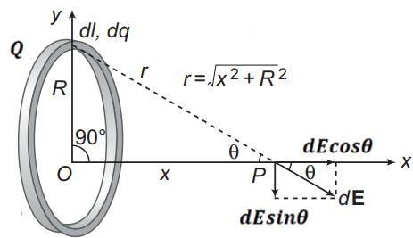
The electric field at point P due to a small charge is
From fig
The net electric field at point P due to the ring is
Special case:
(a) At the centre of the ring x=0 ∴ E=0
(b) For point very close to the centre i.e. x<<R
(c) For point far away from the centre of the ring i.e. x>>R
The ring behaves as a point charge kept at its centre.
(d) For maximum electric field

4. Electric field due to a uniformly charged non-conducting disc on its axis:
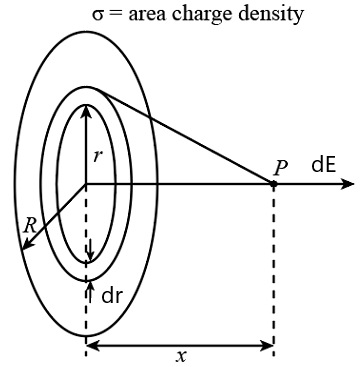
Consider a ring of radius r and thickness dr. The charge on this ring is
The electric field at point P due to this ring is given by
∴ The net electric field at point P due to the disc is
put
Special case
(a) if x>>R
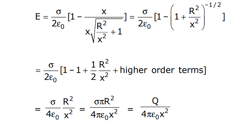
i.e. behaviour of the disc is like a point charge
(b) If x<<R , then we can write
i.e.
i.e. behaviour of the disc is like an infinite sheet of charge
5. Electric field due to charged Hollow hemisphere on its centre:

We know that a hollow sphere is a collection of small rings. If the volume charge density of hollow hemisphere.
Then, from the figure charge on a small ring is
The electric field at the centre due to this ring is
The net electric field at the centre due to the hollow hemisphere is
solve it , we get
Exercise 41. Find the electric field at point P as shown in the figure.
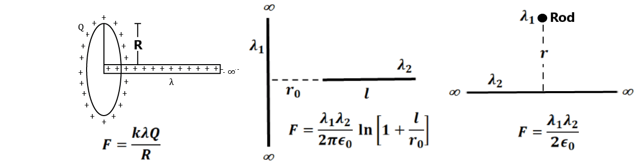
2. Find the force of interaction between the line charge and the ring.
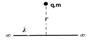
3. A circular wire loop of radius r carries a total charge Q distributed uniformly over its length. A small length dl of the wire is cut off. Find the electric field at the centre due to the remaining wire. 4. Positive charge Q is distributed uniformly over a circular ring of radius R. A particle having a mass m and a negative charge q, is placed on its axis at a distance x from the centre. Find the force on the particle. Assuming x<<R, find the time period of oscillation of the particle if it is released from there. 5. A 10 cm long rod carries a charge of +50μC distributed uniformly along its length. Find the magnitude of the electric field at a point 10 cm from both ends of the rod. 6. A ring of radius R is with a uniformly distributed charge Q on it. A charge q is now placed at the centre of the ring. Find the increase in tension in the ring. 7. If the charge is slightly displaced perpendicular to the wire from its equilibrium position then find out the time period of S.H.M.
|